
GCMSdeco() takes a chromatogram from an ANDI-MS
.cdf file to resolved compound profiles, integrated areas
and a NIST-compatible .msp spectral library. Its
splogconNMF() backend combines sparse selection with local
nonnegative factorization: narrow peaks and broad asymmetric peaks can
each be represented by a single log-concave profile. A smooth background
is fitted jointly, while every original mass channel is retained in the
final spectra.
The single and multichannel deconvolution tutorial introduces selection with a fixed peak shape. Here the peak shapes are refined as part of the factorization, which is particularly useful for overloaded or shark-fin-shaped peaks.
Two experimental chromatograms
The package includes a cuticular-hydrocarbon window with six
co-eluting compounds (GCMS_data1, 119 scans × 671 mass
channels) and a beer-headspace window with a prominent broad acid peak
(GCMS_data2, 1,764 scans × 518 mass channels). Their row
names give retention times in minutes; column names give nominal m/z.
Both examples keep all mass channels.
library(L0glm)
data(GCMS_data1)
data(GCMS_data2)

out <- file.path(tempdir(), "L0glm-GCMS")
dir.create(out, showWarnings = FALSE)
write_GCMS_cdf(GCMS_data1, file.path(out, "GCMS_data1.cdf"))
write_GCMS_cdf(GCMS_data2, file.path(out, "GCMS_data2.cdf"))
write_GCMS_cdf() preserves the intensity matrix,
including silent ions, and writes scan times in seconds for ANDI-MS
readers. The same GCMSdeco() call then works with a matrix
exported from R or a chromatogram exported by instrument software:
fit1 <- GCMSdeco(file.path(out, "GCMS_data1.cdf"),
  file.path(out, "GCMS_data1.msp"), nwindows = 1L, precluster = 16L,
  baseline_df = 1L,
  correlation = "none", ncores = 8L,
  psf_control = list(kernel_est = convkernel("gaussian", 65L,
    list(sigma = 8)), maxiter = 0L))

fit2 <- GCMSdeco(file.path(out, "GCMS_data2.cdf"),
  file.path(out, "GCMS_data2.msp"), nwindows = 1L, precluster = 32L,
  correlation = "none", ncores = 8L,
  psf_control = list(kernel_est = convkernel("gaussian", 65L,
    list(sigma = 6)), maxiter = 0L))

fit1$compounds
GIC(fit2)
coef(fit2, normalize = "l1")       # unit-area spectra in all 518 channels
These short windows use a supplied Gaussian PSF as the initial
profile dictionary. maxiter=0L keeps this PSF fixed;
splogconNMF() then refines the individual compound
profiles. For a full chromatogram, the default nwindows=10L
with positive maxiter estimates a smoothly varying PSF. An
alkane standard can supply its initial calibration through
alkanes_file="alkanes.cdf". The hydrocarbon window uses a
constant background; the longer beer window uses the automatically
chosen low-df cubic spline.
These results were obtained with the calls above on the benchmark workstation, using eight OpenMP workers and one BLAS thread. Timings include CDF reading, PSF initialization, factorization and MSP export.
| Dataset | Scans | Mass channels | Compounds | Time (s) | GIC | Adjusted weighted R² |
|---|---|---|---|---|---|---|
GCMS_data1 |
119 | 671 | 6 | 5.09 | 219,686 | 0.98980 |
GCMS_data2 |
1,764 | 518 | 37 | 58.33 | 1,325,745 | 0.99392 |
Weighted R² uses weights 1/pmax(fitted_mean, 0.1) and a
separate weighted mean for each ion channel. Its adjustment is
conditional on the fitted profiles, using the positive spectral
coefficients and background coefficients as the parameter count.
Cuticular hydrocarbons
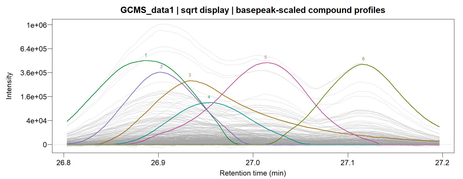
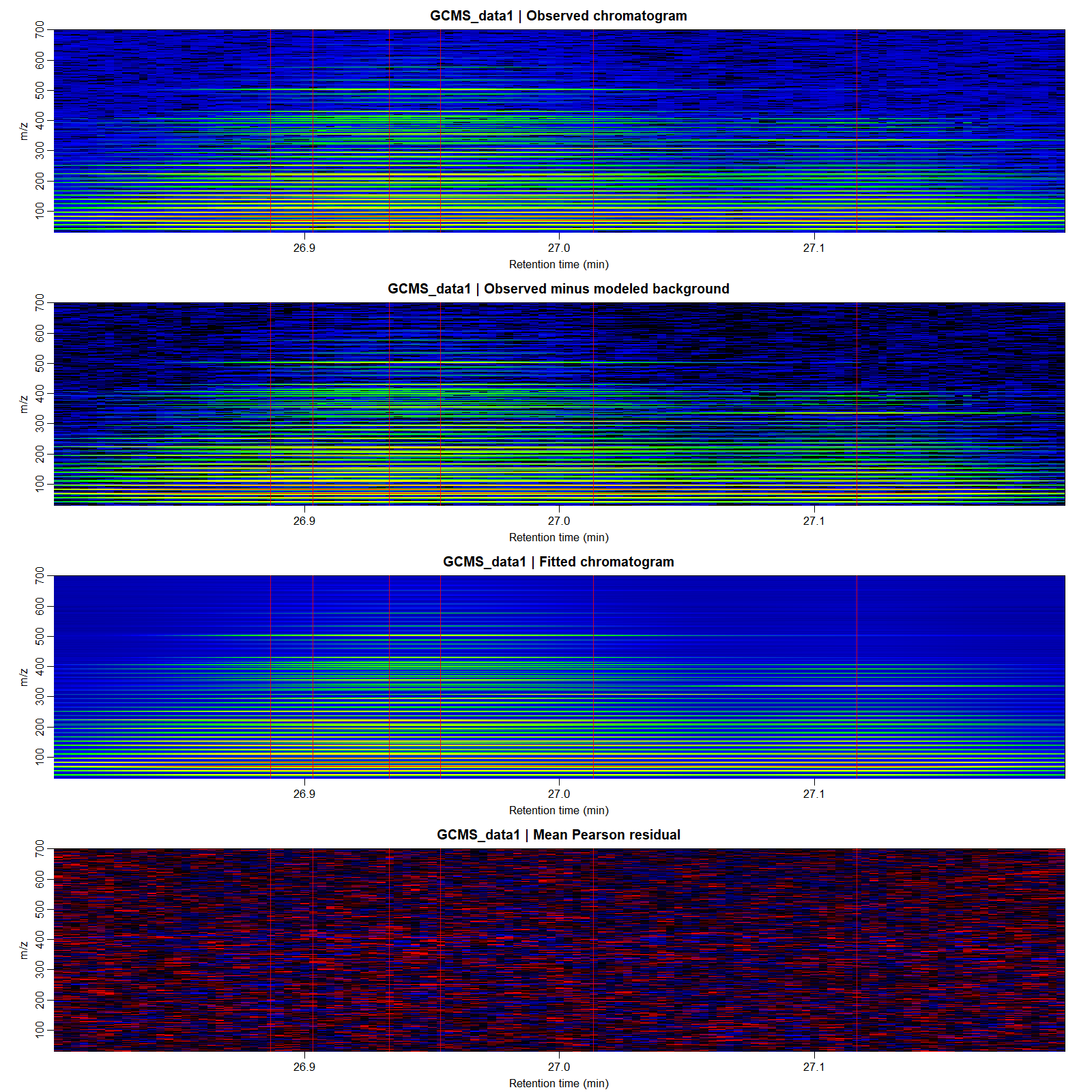
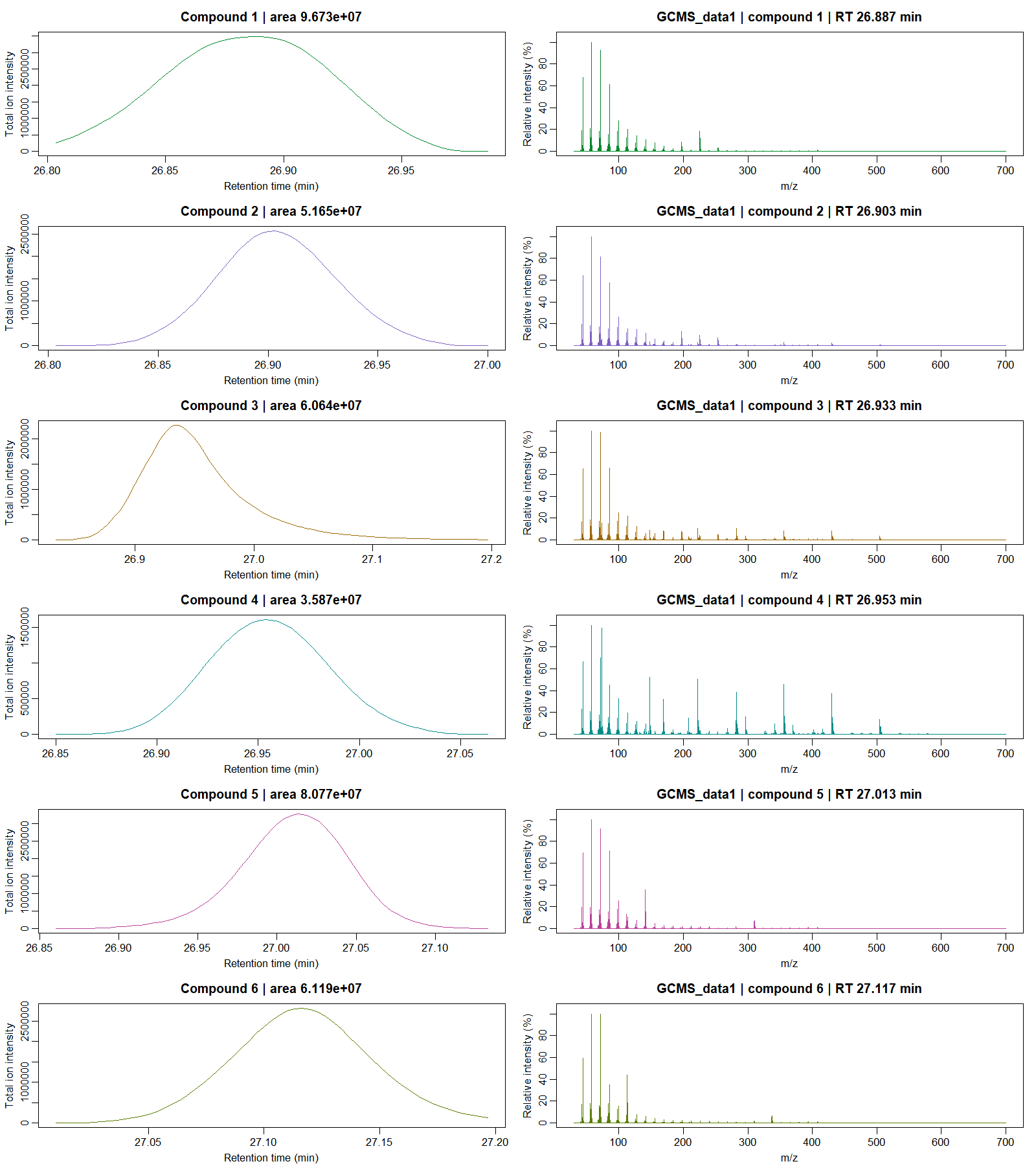
The profile/spectrum panels show every recovered compound.
Download traces, heatmaps, all profiles and spectra, or the MSP library.
Beer volatiles and a broad acid peak
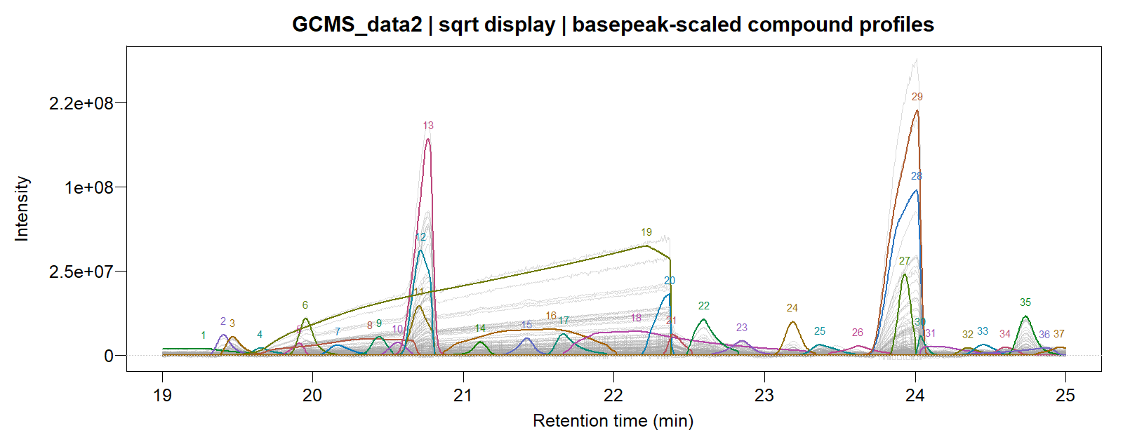
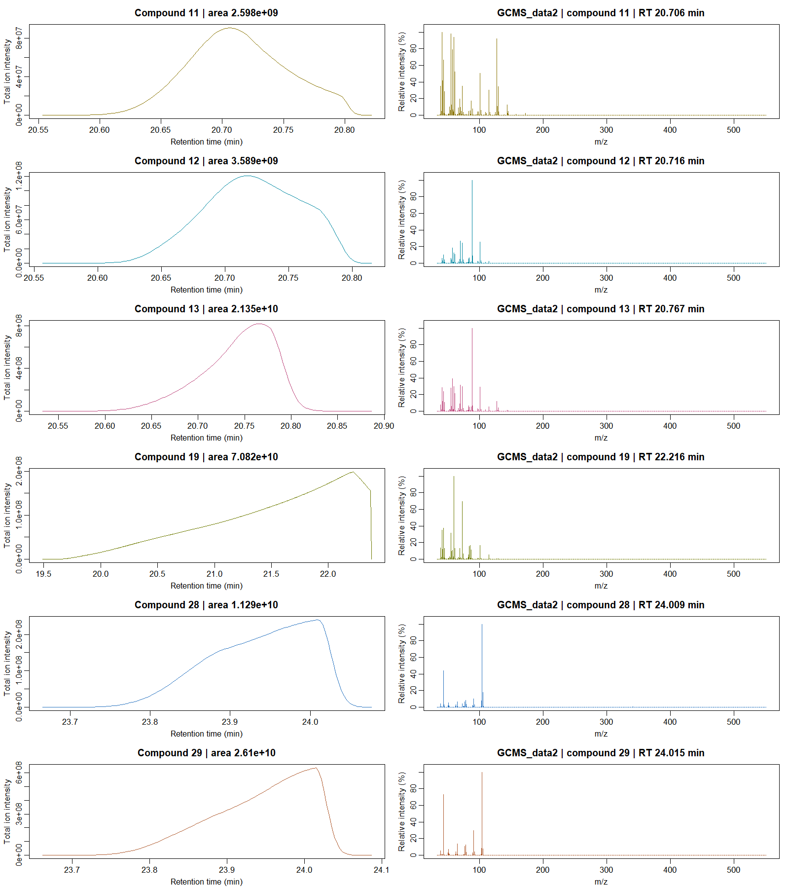
The profile/spectrum preview includes the broadest component and five other large components, in temporal order. The PDF contains every recovered component.
Download traces, heatmaps, all profiles and spectra, or the MSP library.
Plot and export the results
plot(fit1, type = "lines", nrows = 1L,
  minutes_per_panel = diff(range(fit1$time)) + 0.01, labels = TRUE)
plot(fit1, type = "heatmap")
plot(fit1, type = "profiles", nrows = 3L)

plot(fit2, type = "lines", file = file.path(out, "GCMS_data2_traces.pdf"),
  nrows = 1L, minutes_per_panel = diff(range(fit2$time)) + 0.01)
plot(fit2, type = "heatmap", file = file.path(out, "GCMS_data2_heatmaps.pdf"))
plot(fit2, type = "profiles", file = file.path(out, "GCMS_data2_profiles_and_spectra.pdf"),
  nrows = 3L)
Grey traces show individual observed ion signals after subtracting
the fitted background. Coloured curves show the fitted compounds, scaled
by their strongest ion; the square-root display makes weak peaks easier
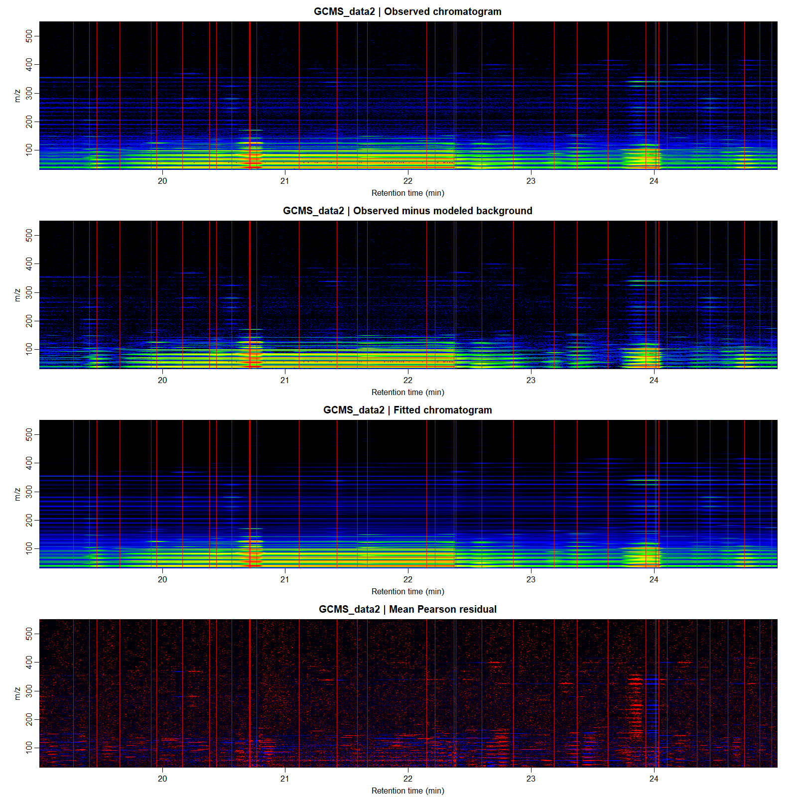
to inspect. The four raster heatmaps show the observations,
background-corrected observations, fitted chromatogram and Pearson
residuals. Red vertical lines mark compound apices. Profile-and-spectrum
panels follow increasing apex retention time; order="area"
displays the largest compounds first.
Supply xlsx_file=file.path(out, "GCMS_data2.xlsx") when
fitting to also export the compound table and integrated areas. Each
spectrum occupies one unwrapped cell, with fragments ordered by
intensity. The returned object stores the source CDF path rather than a
second copy of the observed chromatogram; plotting reloads the required
scans from that file.
Fit a supplied PSF design directly
Use splogconNMF() when a suitable PSF design and
background basis are already available. This also gives direct control
over the background for a short chromatographic window:
Y <- GCMS_data1
X <- convmatrix(convkernel("gaussian", 65L, list(sigma = 8)), nrow(Y))
B <- matrix(1, nrow(Y), 1L)          # constant background in this short window
nmf <- splogconNMF(X, Y, background = B,
  family = quasipoisson("identity"), precluster = 16L,
  correlation = "none", ncores = 8L)
nmf$rank
nmf$H                              # unit-sum, log-concave profiles
coef(nmf)                          # full-channel integrated intensities
GIC(nmf)
For GCMS_data2, a low-dimensional nonnegative spline
background can be constructed with
splines::bs(as.numeric(rownames(Y)), df=4L, intercept=TRUE).
Quasipoisson is useful for instrumental intensities with extra
variation; Poisson, Gaussian, negative binomial and Gamma signal models
are also available. See the likelihood
and shape-constraint details.
Algorithm
For observed scan-by-mass matrix Y, the mean is
\mu=HS+BA+O,\qquad H,S,A\geq0,\qquad \sum_iH_{ir}=1,\quad\Delta^2\log H_{\cdot r}\leq0.
Each column of H is one compound’s
elution profile and each row of S is
its spectrum. The low-df basis B models
background; O is a known offset when
supplied to splogconNMF(). The criterion is
J=-2\sum_{ij}w_{ij}\ell(y_{ij};\mu_{ij},\nu) +m\kappa\lambda_{IC}K,
where K is the compound count, m the original channel count
and \nu the shared noise parameters.
Dividing this criterion by m gives one
rank penalty per compound. Background and profile complexity have no
additional penalty. For quasi families, the likelihood kernel and IC are
scaled by the common dispersion. The optional temporal working
adjustment \kappa=1+2\widehat\rho_1 is
held fixed during rank comparisons; correlation="none" sets
\kappa=1.
- Estimate a shared marginal noise scale from temporal differences, and calibrate the PSF from the sample or an alkane standard.
- Cluster ion traces after adjusting for their total intensity. With
precluster=32L, sum the channels into at most 32 groups. - Fit grouped adaptive ridge on the shifted PSF design and unpenalized background. Fuse spectrally compatible overlapping components when their combined profile is log-concave and the compound-count criterion improves.
- Lift the spectra and background to all original channels. Refit their coefficients using the original observations and noise model.
- Refine local log-concave profiles and spectra, treating all other compounds as offsets. Consider broad-anchor and compatible-tail fusions, restoring distinct components when the full criterion favours them.
- Apply the conservative broad-profile fusion pass, refine the affected neighbourhoods, and return profiles and spectra in temporal order.
The same original-channel compound penalty is used in the reduced-space search. Native Rcpp/OpenMP kernels share the sparse profile design and update only the local scan windows. Candidate clustering uses algebraic spectral and profile calculations; likelihood refits are reserved for proposed model changes and final refinement.
Mathematical background and references
The model is a sparse log-concave nonnegative generalized matrix factorization, with an identity link and a smooth background. Its loss gives the connection to deviance matrix factorization, with rank selection and shape constraints. For standard fixed-parameter exponential-family models its likelihood loss is a weighted Bregman divergence, giving the connection to Bregman NMF. The derivation and noise-specific divergences are given in the mathematical article.
Sparse deconvolution with shifted peak shapes follows the idea of de Rooi & Eilers (2011). Adaptive ridge selection is related to Frommlet & Nuel (2016). Size-adjusted Poisson clustering builds on Witten (2011), while the Poisson likelihood connects to KL-divergence NMF as studied by Lee & Seung (2000). Log-concave profile modelling is inspired by Eilers (2005).
The combination of grouped selection, pooled noise calibration, local original-scale likelihood updates, hard log-concavity and compound-count fusion is developed for L0glm. The sparse log-concave NMF article derives its score, working information, constrained profile updates and likelihood acceptance rules.
The experimental data are described in Van Oystaeyen et al. (2014) and Schreurs et al. (2024).