Model selection and cross-validation

The example below has 1,000 observations, 5,000 predictors and 100 nonzero coefficients of either sign. It shows a rich coefficient path while retaining a genuinely sparse underlying model.

library(L0glm)
sim <- simul("normal", n=1000L, p=5000L, n_nonzero=100L, seed=42L,
  options=list(beta_range=c(-2, 2)))
X <- sim$X
y <- sim$y

A preset or a tuned path

For a single response the sparse-selection target is

-2\ell(\beta) + \lambda\,\|\beta\|_0.

A preset is often a very effective starting point. Searching a path lets the data choose among the candidate sparse models.

fit <- L0glm.fit(X, y, family=gaussian(), lambda="gic", relaxed=TRUE)

Preset	Penalty per selected coefficient
"aic"	2
"bic"	\log n
"gic"	\log p\,\log\log n
"ebic"	\log n + 2\gamma_{\rm EBIC}\log p
"mbic"	\log(np^2/16)

Here p counts selectable predictors, excluding intercepts and mandatory terms. The information-criterion reference gives the parameter-count conventions and literature, including Fan & Tang’s GIC.

gic <- L0glm.tune(X, y, family=gaussian(), tune="gic", nlambda=10L,
  prop_range=.25, relaxed=TRUE, coefs.true=sim$beta_true, plot=TRUE)
c(lambda_best=gic$lambda_best, lambda_preset=gic$lambda_preset)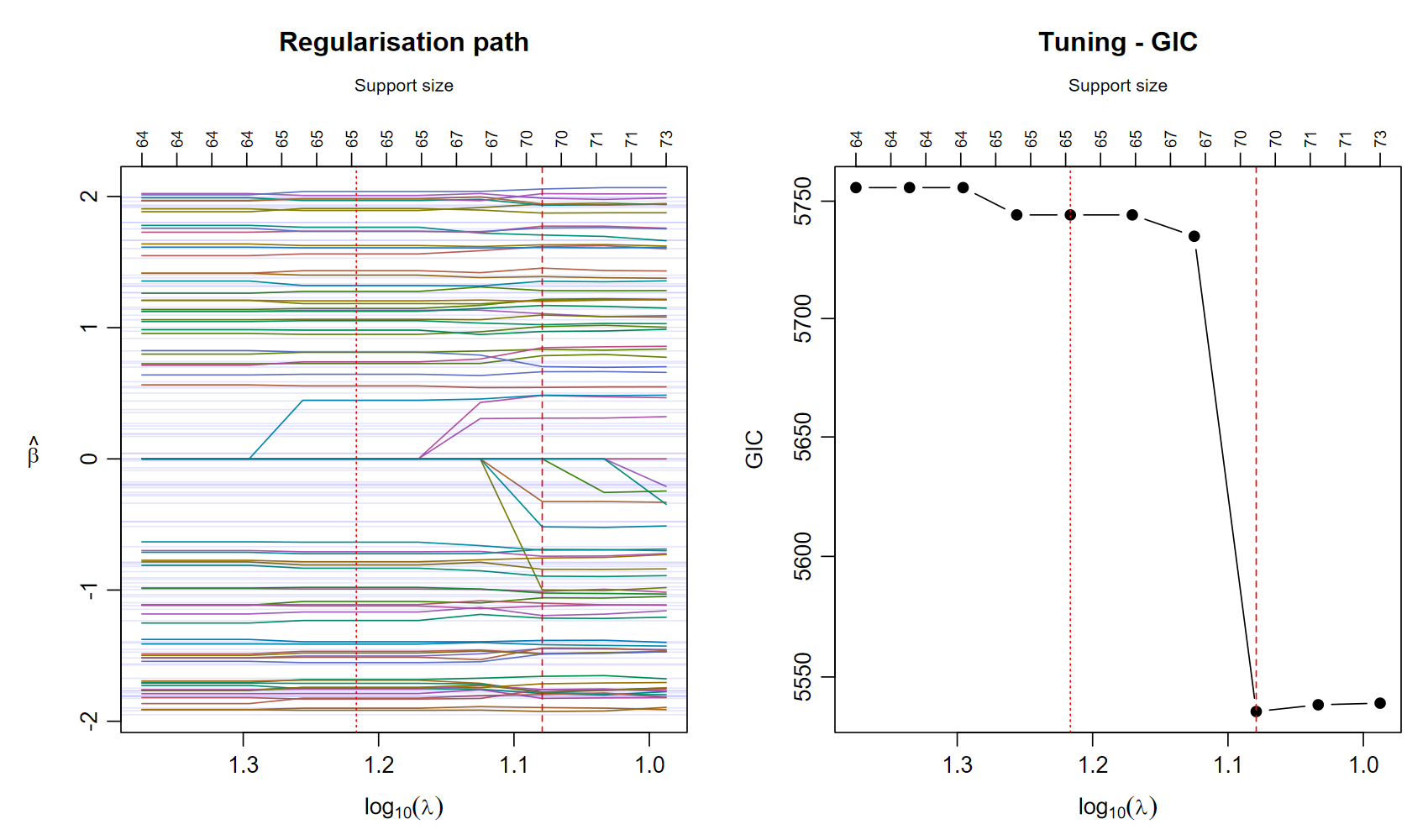

The grid focuses on the preset. Use prop_range=1 to explore the full numerical range. The preset often already gives an excellent model, so detailed path tuning can be reserved for cases where it offers a useful improvement.

Method	GIC	TP	FP	FN	TN	F1	MCC
GIC preset	5744	65	0	35	4900	0.788	0.803
Tuned GIC	5536	70	0	30	4900	0.824	0.834
CV minimum	5539	71	0	29	4900	0.830	0.840
CV one-SE	5744	65	0	35	4900	0.788	0.803

Five-fold cross-validation

CV selects the penalty with the lowest mean held-out deviance. Whole rows are held out, including all response channels. Preprocessing, screening and estimated distribution parameters use the training observations in each fold. The default screen="auto" enables ISIS exactly when p_eligible > 10*n, using the training row count n in that fold. The eligible count excludes mandatory terms and predictors excluded by zero starts in every response channel. There is no separate minimum sample size or predictor count.

set.seed(10)
folds <- sample(rep(1:5, length.out=nrow(X)))
cv <- L0glm.tune(X, y, family=gaussian(), tune="cv", nfolds=5L,
  nlambda=10L, prop_range=.25, foldid=folds, relaxed=TRUE,
  coefs.true=sim$beta_true, plot=TRUE)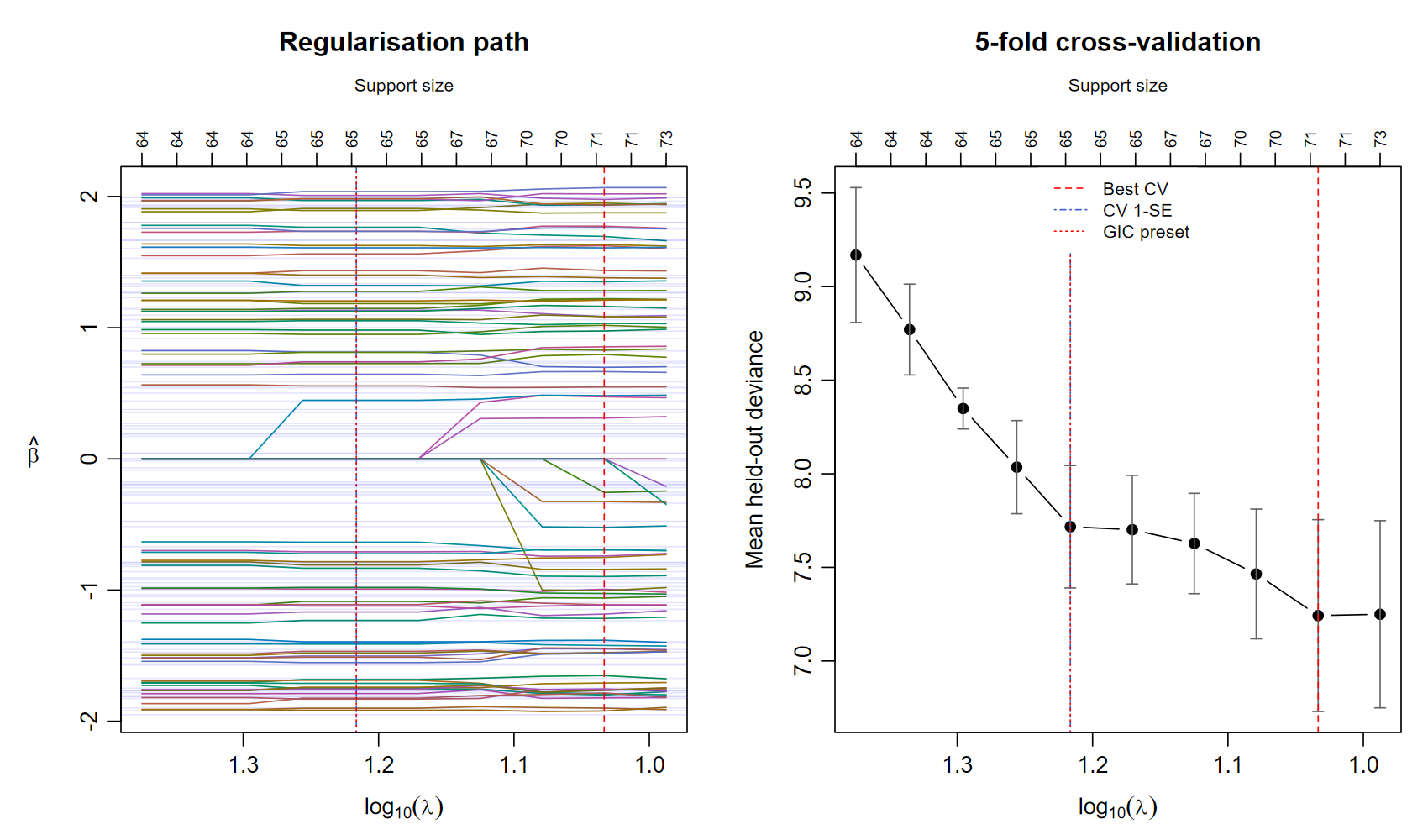

The curves use a reversed log10(lambda) axis: strong regularization is on the left, and support sizes appear above the panels. CV error bars show one standard error.

c(lambda_best=cv$lambda_best, lambda_1se=cv$lambda_1se,
  lambda_preset=cv$lambda_preset)
predict(cv$fit_1se, X[1:5, , drop=FALSE], type="response")

fit_best and fit_1se are full-data fits. The one-SE rule chooses the largest lambda with mean deviance within one SE of the minimum. The GIC preset remains available through lambda_preset for comparison.

Random, contiguous and Venetian-blind folds

Without foldid, folds are randomly assigned. Supply a vector to choose a design:

# Five contiguous blocks
folds <- rep(1:5, length.out=nrow(X))[order(rep(1:5, length.out=nrow(X)))]

# Venetian blind: odd and even observations alternate
folds <- rep(1:2, length.out=nrow(X))
cv <- L0glm.tune(X, y, family=gaussian(), tune="cv",
  foldid=folds, nlambda=10, relaxed=TRUE)

For time-dependent observations, choose folds that reflect how predictions will be used. Reserve an independent test set when measuring final predictive accuracy.

Compare methods

sparseglm() supplies one comparison interface for L0glm, ABESS, L0Learn, LASSO, relaxed LASSO, adaptive variants, MCP and SCAD where supported.

comparison <- sparseglm(X, y, family=gaussian(),
  method=c("L0glm", "abess", "lasso", "relaxed_lasso"),
  tune="cv", nfolds=5, foldid=sample(rep(1:5, length.out=nrow(X))), nlambda=10)
L0glm.metrics(comparison)

method="all" expands to supported methods for the requested model. The benchmark article reports complete fitting and tuning times.