Speed, support recovery and reproducible benchmarks • L0glm

L0glm’s shrinking active set, compiled solvers and fast GIC preset can deliver striking gains in both speed and support recovery. These examples compare complete fitting and selection workflows, with the tuning rule stated for every method. The realistic deconvolution examples are generated by the website benchmark. The million-predictor comparison reproduces the LASSO workflows. The README and this page share the same published measurements.

One million predictor example

The design has 500 observations, one million standard-normal predictors and 60 nonzero coefficients of either sign. L0glm uses GIC-preset ISIS plus a relaxed refit. LASSO and fully relaxed LASSO are tuned by BIC or five-fold CV.

Method	Selection	Seconds	GIC	TP	FP	FN	TN	F1	MCC
L0glm + ISIS	GIC preset	3.49	2583	40	3	20	999937	0.777	0.787
LASSO	BIC path	22.75	14789	23	612	37	999328	0.066	0.118
Relaxed LASSO	BIC path	21.42	10588	21	453	39	999487	0.079	0.124
LASSO	5-fold CV	123.13	4309	17	50	43	999890	0.268	0.268
Relaxed LASSO	5-fold CV	91.76	7413	20	252	40	999688	0.120	0.156

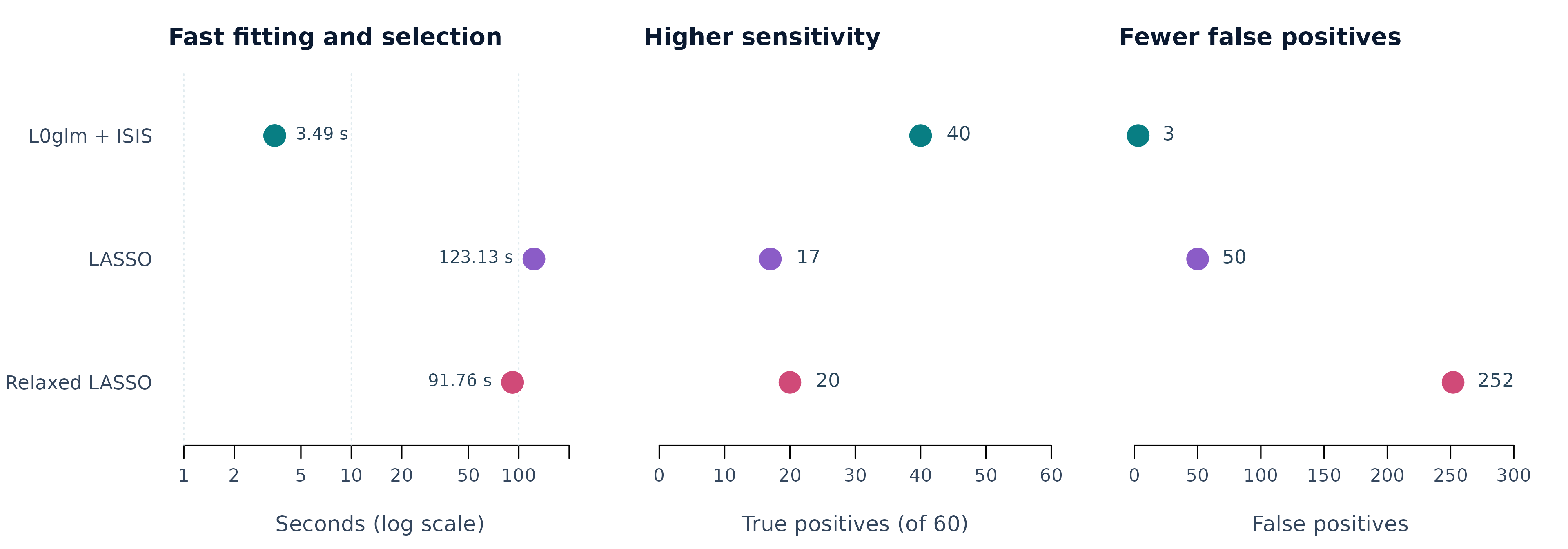
Fast fitting and selection, higher sensitivity and fewer false positives in the million-predictor example. L0glm uses a GIC preset; both LASSO methods use five-fold CV. There are 60 true effects.

In this simulation L0glm is 35 times faster than five-fold-CV LASSO and recovers more true effects with fewer false positives. The L0glm timing includes screening and one preset fit; the other methods evaluate up to 40 native path values, with paths refitted in each CV training fold. BIC is shown alongside CV because GIC can select a null LASSO model at this dimension. All rows retain GIC as a common evaluation score. Five-fold comparisons use the same random folds.

Simulation is excluded from timings. The documented run uses one BLAS thread and eight screening threads; the design is held in memory. The L0glm time is the median of three runs. The common-scoring CV implementation used for the LASSO rows evaluates folds serially. Standalone benchmarks that call cv.glmnet() use parallel folds through cv_glmnet_parallel(). See the million-predictor tutorial for the complete data setup.

Single channel deconvolution

A realistic blurred Poisson spike train has 10,000 observations, 10,000 predictors and 1,000 true peaks. Every fit is evaluated using the original Poisson likelihood and a common GIC.

Method	Selection	Seconds	GIC	TP	FP	FN	TN	F1	MCC
L0glm	GIC preset	0.20	102682	845	154	155	8846	0.845	0.828
LASSO	GIC path	0.40	145904	950	2096	50	6904	0.470	0.467
Relaxed LASSO	GIC path	0.64	122083	905	999	95	8001	0.623	0.607
LASSO	5-fold CV	4.83	146234	951	2146	49	6854	0.464	0.462
Relaxed LASSO	5-fold CV	6.70	133122	920	1523	80	7477	0.534	0.524

L0glm uses one GIC preset with a relaxed refit. LASSO and relaxed LASSO search ten explicit lambda values using GIC or five-fold CV, with a weighted-Gaussian approximation and observation weights 1/(y+0.1). CV selects glmnet’s minimum weighted prediction error using four parallel workers. ABESS is omitted from this large example. The deconvolution tutorial shows mirrored signals and true-versus-estimated coefficient plots.

Multichannel deconvolution

The GC/MS-style simulation also has 10,000 rows, 10,000 candidate peak locations and 1,000 true peaks, with all 226 informative mass channels retained. Shared chromatographic peak times correspond to active coefficient rows; within-row coefficients describe the mass spectra.

Method	Selection	Seconds	GIC	TP	FP	FN	TN	F1	MCC	Within-row F1	Within-row MCC
L0glm	GIC preset	9.63	5615963	944	11	56	8989	0.966	0.962	0.909	0.864
Group LASSO	GIC path	244.87	7413616	980	860	20	8140	0.690	0.685	0.842	0.768
Relaxed group LASSO	GIC path	906.34	6138687	909	309	91	8691	0.820	0.802	0.853	0.782
Group LASSO	5-fold CV	813.42	9639345	998	4242	2	4758	0.320	0.316	0.886	0.830
Relaxed group LASSO	5-fold CV	3199.62	6198648	962	502	38	8498	0.781	0.769	0.856	0.785

Row F1 and MCC measure peak recovery. Within-row F1 and MCC assess spectral sparsity among correctly recovered true-positive peaks. L0glm uses the full Poisson likelihood with channel-specific working weights. Grouped glmnet uses shared row weights 1/(rowMeans(y)+0.1) for its labelled Gaussian approximation. GIC selection scores ten lambda values using the original Poisson likelihood; five-fold CV selects the minimum weighted prediction error on the same lambda grid. Fully relaxed fits use gamma=0. L0glm uses lambda="gic" and four outcome-fitting threads; CV uses four parallel workers. Timings include the complete fitting and selection workflow, including worker startup for CV. The preset time is the median of three runs with matching coefficients. Simulation and final metric reporting are excluded.

The deconvolution tutorial stacks observed data, ground truth and fitted coefficient heatmaps, and shows all-channel coefficient comparisons in a single column.

Native validation and OpenMP

Native validation scoring preserves multichannel OpenMP and returns the same checkpoint models as the R-validation path. This reproducible test uses 1,000 predictors, 16 channels, 60 active rows and an independent Poisson replicate for validation. Median times are from five fits, with one BLAS thread.

Backend	Outcome threads	Seconds	Validation deviance	GIC	F1	MCC
General R	1	1.12	0.357612	42728.05	0.944882	0.942790
Native	1	0.08	0.357612	42728.05	0.944882	0.942790
Native	2	0.06	0.357612	42728.05	0.944882	0.942790
Native	4	0.04	0.357612	42728.05	0.944882	0.942790
Native	8	0.04	0.357612	42728.05	0.944882	0.942790

Run benchmark_native_validation.R to reproduce this comparison. Results agree across thread counts; validation predictors are shared across workers. Paired 10,000-predictor tests also preserve the unvalidated fit, with 16-channel timing 0.874 s versus 0.878 s.

Reproduce and extend

Website benchmark source: preset fits, comparisons and plots.
Million-predictor LASSO benchmark: BIC and five-fold CV comparisons.
Solver/problem-size benchmark: solvers, families, matrix storage and sizes.
Single/multichannel benchmark: detailed signal examples and alternative methods.
sparseglm(): use the same comparison framework on your own data.

The benchmarks were run on an HP ZBook Fury 17.3-inch G8 Mobile Workstation with an 11th-generation Intel Core i9-11950H at 2.60 GHz, 8 physical cores and 16 logical cores, running Windows and R 4.5.0 with OpenBLAS. BLAS uses one thread. Screening in the million-predictor example uses eight physical cores. Multichannel deconvolution uses four outcome-fitting threads, and deconvolution CV uses four parallel workers. Single-channel fits use one fitting thread. Timings will vary with hardware and tuning choices. F1 and MCC evaluate the known simulated support; it is never used to select models. Likelihood floors and approximation labels are explicit in the benchmark source.