Poisson spike-train deconvolution

The L0 deconvolution idea was inspired by work by de Rooi & Eilers (2011). Our methods for automatically setting regularization, the extensions to Poisson or negative-binomial noise, and the multichannel shared-support extensions are new developments of the present work. simul() supports all three noise models.

In deconvolution, a design matrix contains shifted copies of the peak-shape function, also called the point spread function. Sparse coefficients represent sharp events, while the measured signal is blurred and noisy. For nonnegative Poisson intensities,

Y_i\sim\operatorname{Poisson}\{(X\beta)_i\},\qquad\beta\geq0.

The following examples each have 10,000 observations, 10,000 candidate peak locations and 1,000 true peaks. L0glm fits the Poisson likelihood directly; the native OpenMP backend shares the sparse convolution design across channels. L0glm uses the GIC preset. Competing LASSO methods use ten lambda values, selected by GIC or native five-fold CV with weighted prediction error. See benchmark hardware and timing conventions.

Single channel deconvolution

library(L0glm)
single <- simul(method=2L, n=10000L, p=10000L,
  n_nonzero=1000L, seed=2L)
system.time(fit <- L0glm.fit(single$X, single$y, family=poisson("identity"),
  lambda="gic", nonnegative=TRUE, intercept=FALSE, relaxed=TRUE,
  parallelize=TRUE, ncores=4L))
L0glm.metrics(fit, beta_true=single$beta_true)[c("gic", "TP", "FP", "FN", "TN",
  "F1_score", "MCC")]

L0glm recovers 845 of 1,000 true peaks with just 154 false positives in 0.20 seconds: 2× faster than GIC-tuned LASSO and 34× faster than relaxed LASSO tuned by five-fold CV in this comparison.

Method	Selection	Seconds	GIC	TP	FP	FN	TN	F1	MCC
L0glm	GIC preset	0.20	102682	845	154	155	8846	0.845	0.828
LASSO	GIC path	0.40	145904	950	2096	50	6904	0.470	0.467
Relaxed LASSO	GIC path	0.64	122083	905	999	95	8001	0.623	0.607
LASSO	5-fold CV	4.83	146234	951	2146	49	6854	0.464	0.462
Relaxed LASSO	5-fold CV	6.70	133122	920	1523	80	7477	0.534	0.524

The table compares the GIC-preset fit with LASSO and fully relaxed LASSO, each selected by GIC or five-fold CV over the same ten-value lambda grid. The GIC comparison is available through sparseglm():

gic <- sparseglm(single, family=poisson("identity"),
  method=c("lasso", "relaxed_lasso"), tune="gic", nlambda=10L,
  nonnegative=TRUE, intercept=FALSE, approximation="wls")

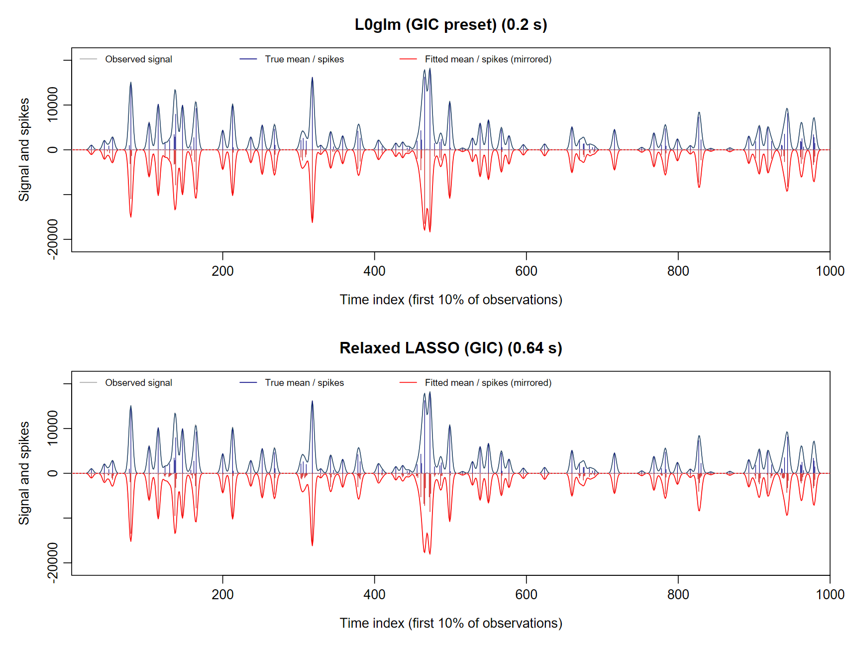
The observed and true signal are shown above zero; fitted signals and estimated spikes are mirrored below in red. These panels zoom into the first 1,000 time points, using the same vertical scale for both methods. They compare L0glm with the strongest competing method in this example, ranked by support MCC.

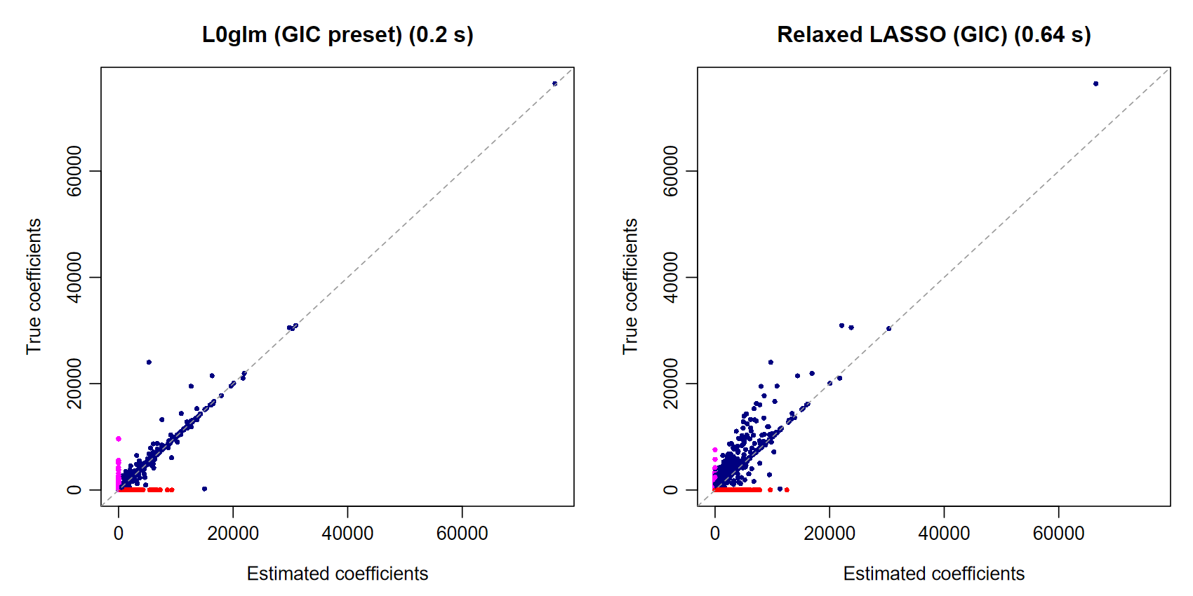
The coefficient comparison retains all 10,000 predictors and shows estimation accuracy and the additional coefficients selected by the competing method. Each common (0,0) is plotted once.

Multichannel deconvolution

Gas chromatography–mass spectrometry (GC/MS) provides a natural application: compounds with overlapping chromatographic peaks contribute counts across many mass-to-charge channels. Peak locations are shared across channels, while each compound has its own sparse mass spectrum. A grouped Poisson model recovers the peak locations and the corresponding spectra together.

The simulation retains all 226 informative mass channels generated from the spectral library. No channels are discarded for fitting or plotting.

multi <- simul(method=4L, n=10000L, p=10000L,
  n_nonzero=1000L, seed=2L)
system.time(fit_multi <- L0glm.fit(multi$X, multi$y, family=poisson("identity"),
  lambda="gic", nonnegative=TRUE, intercept=FALSE, grouped=TRUE, relaxed=TRUE,
  parallelize=TRUE, ncores=4L))
L0glm.metrics(fit_multi, beta_true=multi$beta_true)[c("gic", "TP", "FP", "FN", "TN",
  "F1_score", "MCC", "within_row_F1_score", "within_row_MCC")]

L0glm recovers 944 of 1,000 true peaks with just 11 false positives in 9.63 seconds: 25× faster than GIC-tuned group LASSO and 332× faster than relaxed group LASSO tuned by five-fold CV in this comparison.

Method	Selection	Seconds	GIC	TP	FP	FN	TN	F1	MCC	Within-row F1	Within-row MCC
L0glm	GIC preset	9.63	5615963	944	11	56	8989	0.966	0.962	0.909	0.864
Group LASSO	GIC path	244.87	7413616	980	860	20	8140	0.690	0.685	0.842	0.768
Relaxed group LASSO	GIC path	906.34	6138687	909	309	91	8691	0.820	0.802	0.853	0.782
Group LASSO	5-fold CV	813.42	9639345	998	4242	2	4758	0.320	0.316	0.886	0.830
Relaxed group LASSO	5-fold CV	3199.62	6198648	962	502	38	8498	0.781	0.769	0.856	0.785

Row F1 and MCC measure recovery of peak times. Within-row F1 and MCC measure mass-spectrum sparsity among correctly recovered true-positive peaks. Group LASSO and relaxed group LASSO use glmnet’s grouped Gaussian approximation, with shared row weights 1/(rowMeans(y)+0.1); every selected model is evaluated using the original Poisson likelihood and the same GIC. Each glmnet path has ten lambda values. Relaxed group LASSO refits the selected shared row support with gamma=0. Native cv.glmnet() selects the minimum weighted prediction error using five common random folds and four parallel workers. L0glm uses a single GIC preset with four outcome-fitting threads. CV timings include worker startup and the full-data refit; simulation and final metric reporting are excluded. The L0glm time is the median of three fits with matching coefficients.

gic_multi <- sparseglm(multi, family=poisson("identity"),
  method=c("lasso", "relaxed_lasso"), tune="gic", nlambda=10L,
  nonnegative=TRUE, intercept=FALSE, approximation="wls_grouped")

The benchmark source reproduces both selection rules, the timings and every reported metric.

Correlated peaks and group LASSO

Shifted copies of the point-spread function are strongly correlated. For this design, the standard group-LASSO irrepresentability diagnostic is 20.54, well above the bound of one. This helps explain why group LASSO can retain many neighbouring peak locations even while reconstructing the observed signal well. L0glm’s direct support penalty gives a much cleaner separation of the peaks.

To compute the diagnostic, let A be the shared-row-weighted design with columns scaled to unit norm, S the true row support and U_{j\cdot}=B^*_{j\cdot}/\|B^*_{j\cdot}\|_2. We evaluate

\max_{j\notin S}\left\| A_j^\top A_S(A_S^\top A_S)^{-1}U_S \right\|_2.

For ordinary group LASSO, the corresponding population quantity must be at most one to achieve consistent coefficient estimation together with exact group-support recovery; a strict inequality gives a sufficient condition under the assumptions of Bach (2008), Theorems 2–3. If that population condition remains violated, increasing the sample size alone cannot make the probability of recovering the true groups tend to one while also consistently estimating their coefficients, whatever regularization sequence is used. Strong predictor dependence can therefore remain an obstacle even with extremely large datasets.

The value above is a fixed-design diagnostic for the unconstrained weighted-Gaussian group model; the benchmark additionally uses nonnegativity constraints and Poisson scoring. The diagnostic script gives the calculation and numerical solve check.

Reference: Bach, F. R. (2008). Consistency of the Group Lasso and Multiple Kernel Learning. Journal of Machine Learning Research, 9, 1179–1225.

Compare the recovered signals and spectra

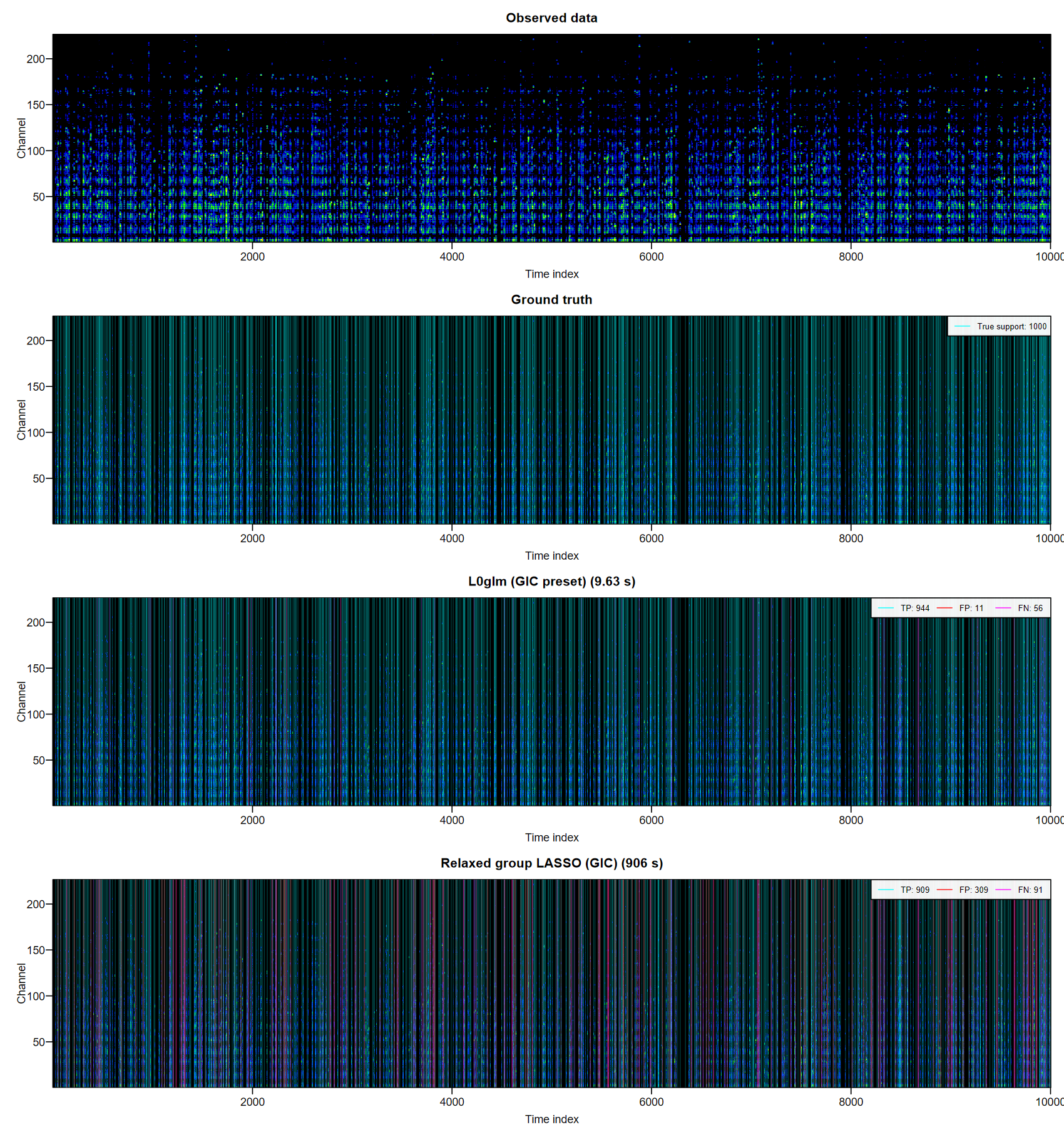
Heatmaps stack the observed data, ground-truth coefficients and selected methods on one page. Coefficient panels share a colour scale; observed counts have their own intensity scale. Cyan overlays mark true support or true positives, red marks false positives and magenta marks false negatives. Legends also give the counts. Every channel is retained.

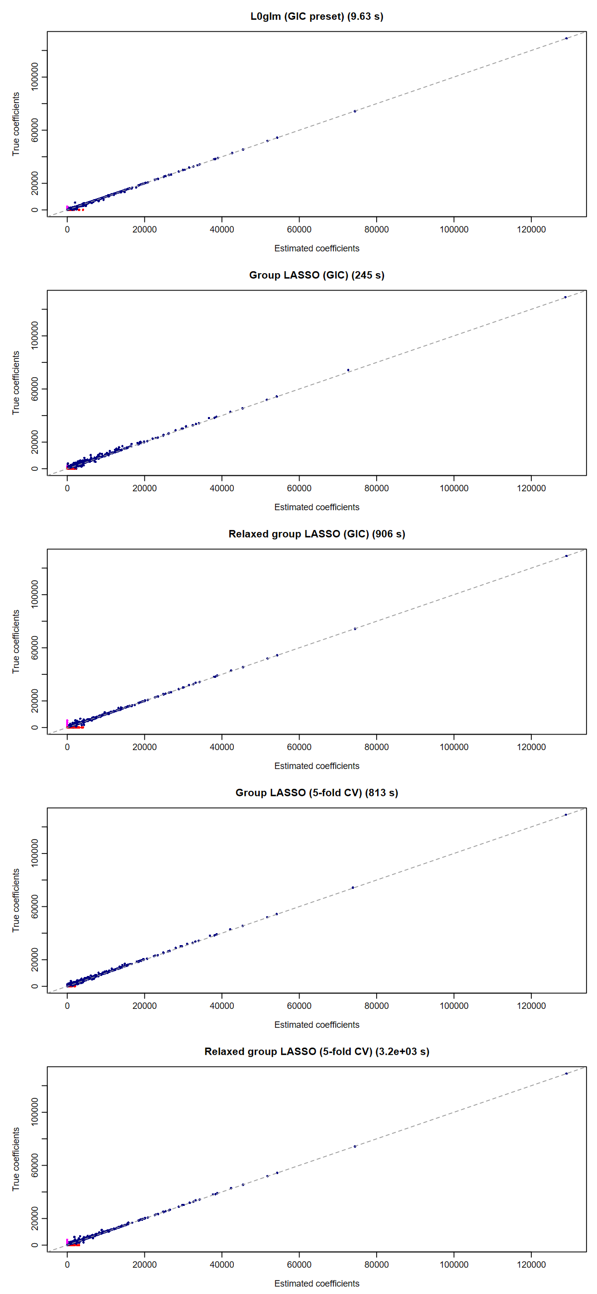
Multichannel true-versus-estimated coefficient panels use a single column. Blue points are correctly recovered nonzero coefficients, red points are false positives and magenta points are false negatives.

Cluster channels for faster support selection

For multichannel nonnegative Poisson models, precluster=TRUE first clusters and sums channels, selects promising peak locations in that reduced problem, then refines the fit on every original channel. cluster.refit=FALSE instead returns coefficients for the summed cluster outcomes.

Both Ward and Bregman clustering use channel totals as size factors, size_fac=colSums(Y). This accounts for differences in overall ion intensity while comparing the shapes of the chromatographic traces. The regression stages use the raw counts. Ward uses a smoothed Poisson dissimilarity; Bregman merges groups using their actual pooled Poisson likelihood loss.

clustered <- L0glm.fit(multi$X, multi$y, family=poisson("identity"),
  lambda="gic", nonnegative=TRUE, grouped=TRUE, relaxed=TRUE,
  precluster=TRUE,
  control.precluster=list(linkage="ward", rowbins=5L, k.max=32L))
clustered$preclustering$seconds
L0glm.metrics(clustered, beta_true=multi$beta_true)[c(
  "gic", "F1_score", "MCC", "within_row_F1_score", "within_row_MCC")]

Five-scan binning speeds up clustering of these ordered traces; fitting retains every scan. linkage="bregman" provides the alternative likelihood-based hierarchy with the same size factors. For CV, memberships and size factors are learned separately in each training fold. See channel preclustering for controls, starting values and aggregate-only output.

A smooth nonnegative background

For a full chromatogram, add a low-df B-spline basis to describe the slowly varying background. Keeping these columns in always.include leaves them unpenalized. L0glm alternates a small constrained background solve with sparse peak fitting, using every original mass channel. For Poisson identity models, the spline contribution is directly additive in signal units.

B <- splines::bs(seq(0, 1, length.out=nrow(multi$X)), df=6, intercept=TRUE)
Z <- cbind(multi$X, Matrix::Matrix(B, sparse=TRUE))
compulsory <- ncol(multi$X) + seq_len(ncol(B))
background_fit <- L0glm.fit(Z, multi$y, family=poisson("identity"),
  lambda="gic", nonnegative=TRUE, always.include=compulsory,
  grouped=TRUE, relaxed=TRUE, precluster=TRUE,
  control.precluster=list(k.max=32L, rowbins=5L))
background <- B %*% as.matrix(coef(background_fit)[compulsory, , drop=FALSE])
peak_coefficients <- coef(background_fit)[seq_len(ncol(multi$X)), , drop=FALSE]
background_fit$nuisance$seconds

The same compulsory-block approach supports Gaussian and negative-binomial models and other scalar GLM links. The background is additive on the chosen link scale. Automatic channel aggregation remains specific to nonnegative identity-link Poisson models. See compulsory terms and backgrounds for the equations, constraints and initialization.

Regularization and tuning

An automatically preset level of regularization with lambda="gic" typically provides a near-optimal sparse solution straight away. Tuning over a lambda grid or cross-validation remains available to refine regularization further or optimize out-of-sample predictive performance.

gic <- L0glm.tune(multi$X, multi$y, family=poisson("identity"),
  tune="gic", nlambda=10L, nonnegative=TRUE, grouped=TRUE, relaxed=TRUE)
cv <- L0glm.tune(multi$X, multi$y, family=poisson("identity"),
  tune="cv", nfolds=5L, nlambda=10L, nonnegative=TRUE, grouped=TRUE, relaxed=TRUE)

See the full benchmark tables for the preset and tuned fits.