SPARSE REGRESSION · GENERALIZED LINEAR MODELS

Fast variable selection.
Parsimonious models.

Fast L₀ and grouped L₀ regression to approximate best subset and best subset of groups selection. Accurate effects, cleaner supports, and one interface from ordinary GLMs to multinomial and survival models.

Get started Explore the benchmarks

R · Dense & sparse designs · Single & multiple responses

1 millionpredictors in a high dimensional example 35× fasterthan five-fold-CV LASSO in that example 944 / 1000peaks recovered in multichannel GC/MS deconvolution and 94× faster than relaxed group LASSO

Sparse learning across a wide range of models

L0glm combines adaptive ridge with iteratively reweighted least squares, fast linear solvers and an optional relaxed refit. Small effects drop out; strong effects retain their magnitude. A shrinking active set concentrates computation where it matters, producing sparse models with excellent support recovery.

01 / MODELS

One fitting interface

Gaussian, Poisson, binomial, Gamma and inverse Gaussian GLMs; negative binomial with estimated shape; joint multinomial regression; and Cox proportional hazards.

02 / SCALE

Built for sparse signals

Dense or sparse matrices, tall or wide systems, grouped multichannel selection, and compiled SIS/ISIS screening for ultrahigh dimensions.

03 / CONTROL

Fit the model you need

Observation weights, offsets, nonnegative coefficients, unpenalized terms, normalization and original-scale estimates. Native OpenMP accelerates nonnegative identity-link Poisson fits.

04 / SELECTION

Choose your workflow

Start with a fast GIC preset, tune an information criterion, or use cross-validation with minimum-deviance and one-standard-error models. Compare methods with sparseglm().

Fit a sparse model

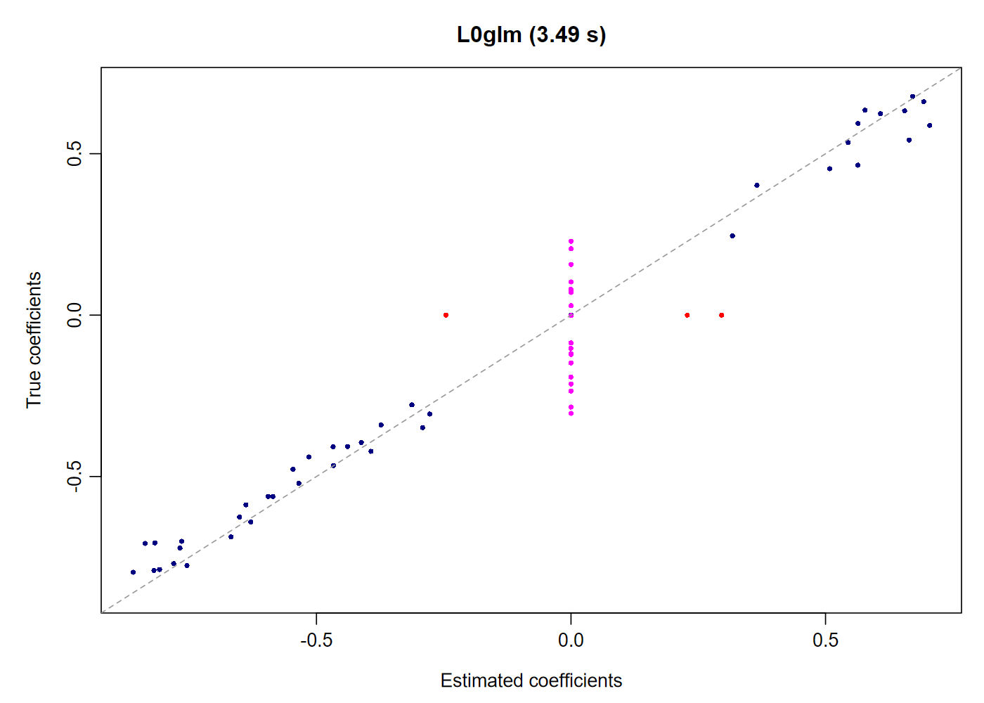
Sixty nonzero effects among one million predictors, fitted in one simple call in about 3 seconds, with 40 out of 60 successfully recovered and just 3 false positives:

library(L0glm)
set.seed(123)
n <- 500L
p <- 1000000L
X <- matrix(rnorm(n*p), n, p)
active <- sample.int(p, 60L)
beta <- numeric(p)
beta[active] <- runif(60L, -.8, .8)
set.seed(1)
y <- as.numeric(X[, active] %*% beta[active]) + rnorm(n)

system.time(fit <- L0glm.fit(X, y, family=gaussian()))
L0glm.metrics(fit, beta_true=beta)[
  c("gic", "TP", "FP", "FN", "TN", "F1_score", "MCC")]

Seconds	GIC	TP	FP	FN	TN	F1	MCC
3.49	2583	40	3	20	999937	0.777	0.787

Recovered coefficients show near-zero bias:

Recovered versus true effects in the million-predictor example.

Install with remotes::install_github("tomwenseleers/L0glm", subdir="L0glm"). The dense design occupies about 4 GB. The getting-started guide explains the example and prediction methods.

Application: sparse deconvolution

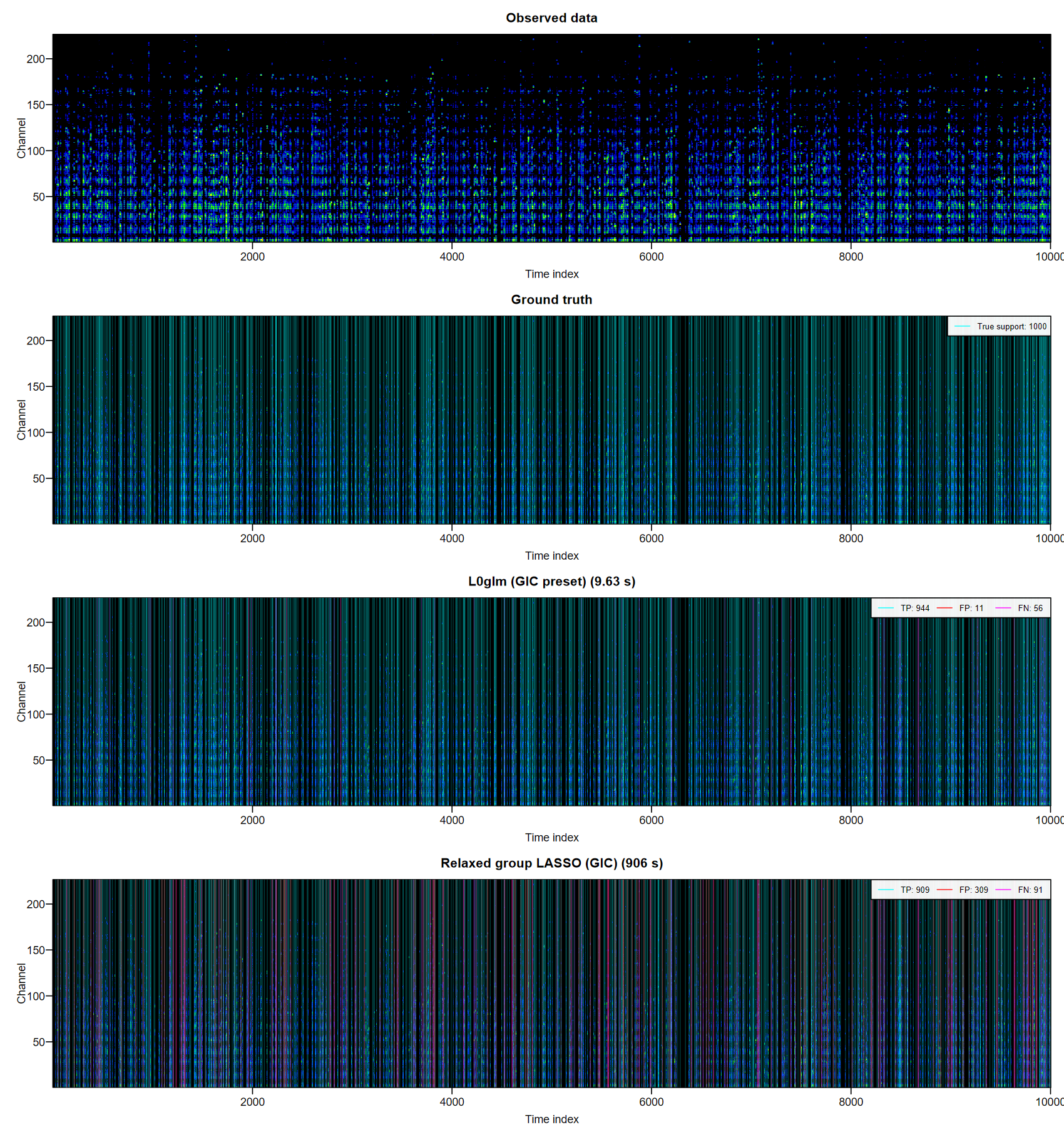
In GC/MS analysis, overlapping chromatographic peaks have distinct mass spectra. Recovering their peak times and spectra together is a natural application of grouped L₀ regression. This Poisson simulation has 10,000 observations, 10,000 candidate peak locations, 1,000 true peaks and 226 mass channels.

By regressing the observed signal on a design matrix consisting of shifted copies of the peak-shape function (the point spread function), L0glm recovers the underlying peaks and their mass spectra.

L0glm recovers 944 of 1,000 true peaks with just 11 false positives in 9.63 seconds: 25× faster than GIC-tuned group LASSO and 332× faster than relaxed group LASSO tuned by five-fold CV in this comparison. It also recovers the sparse mass spectra accurately, with a within-row F1 of 0.909. A direct L0glm.fit() call uses lambda="gic" and four cores; the competing methods select lambda from a ten-value grid using GIC or five-fold cross-validation.

multi <- simul(method=4L, n=10000L, p=10000L,
  n_nonzero=1000L, seed=2L)
fit_multi <- L0glm.fit(multi$X, multi$y, family=poisson("identity"),
  lambda="gic", nonnegative=TRUE, ncores=4L)

Method	Selection	Seconds	GIC	TP	FP	F1	MCC
L0glm	GIC preset	9.63	5615963	944	11	0.966	0.962
Group LASSO	GIC path	244.87	7413616	980	860	0.690	0.685
Relaxed group LASSO	GIC path	906.34	6138687	909	309	0.820	0.802
Group LASSO	5-fold CV	813.42	9639345	998	4242	0.320	0.316
Relaxed group LASSO	5-fold CV	3199.62	6198648	962	502	0.781	0.769

Multichannel GC/MS peak recovery: observed data, ground truth, L0glm and relaxed group LASSO, retaining all 226 channels. Cyan lines mark true positives, red false positives and magenta false negatives.

The coefficient comparison shows how closely L0glm recovers the individual mass-spectral intensities. Relaxed group LASSO is the strongest alternative in this benchmark.

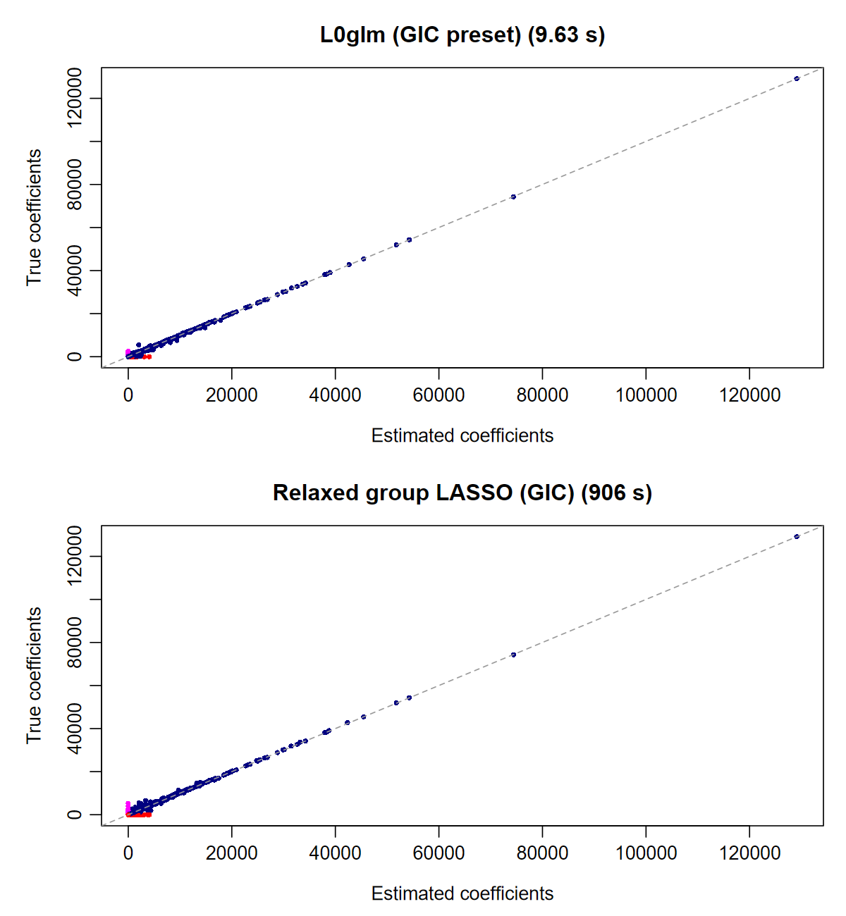
True versus estimated coefficients across all channels for L0glm and relaxed group LASSO.

L0glm fits the Poisson model directly. The group-LASSO methods use a weighted-Gaussian approximation with shared observation weights; CV uses four parallel workers. Explore the deconvolution examples and full benchmark tables →

For broad or asymmetric peaks, splogconNMF() recovers log-concave elution profiles and spectra with a smooth background. GCMSdeco() runs the workflow directly from an ANDI-MS .cdf chromatogram and exports the compound spectra to a NIST-compatible .msp library.

Choose a starting point

I would like to…	Start here
Fit a model and make predictions	Get started
Choose a penalty by GIC or cross-validation	Model selection
Use weights, constraints or held-out early stopping	Fitting controls
Fit counts, classes or survival outcomes	Negative binomial · Multinomial · Cox
Search a very large predictor set	SIS / ISIS
Understand the mathematics	Algorithm & theory
Compare speed and support recovery	Benchmarks

Foundations

The method builds on adaptive ridge and broken adaptive ridge, with an IRLS implementation for generalized linear models. The algorithm article develops the quadratic updates and their connection to sparse penalties, drawing on Frommlet & Nuel (2016), Li et al. (2021) and Abergel, Bouaziz & Nuel (2024). It also explains screening, grouped selection and likelihood-based scoring. The adaptive updates also have a hierarchical Bayesian and automatic relevance determination (ARD) interpretation: each ridge step estimates a Gaussian-prior MAP, then the prior scales adapt to the fitted effects. Zero-centered skeptical priors tighten around small effects and relax around strong ones.

Citation

An article describing the methods implemented in L0glm is in preparation. If you use the package before the article is formally published, we would appreciate a citation to the package:

Wenseleers T, Lanzas L, Vanderaa C (2026). L0glm: Fast Sparse Regression for Generalized Linear Models. R package version 0.1.0, https://tomwenseleers.github.io/L0glm/.

The Authors and Citation page also provides the citation in BibTeX format.

Acknowledgements

OpenAI Codex, using GPT-6 Astra and GPT-6.1 Sol, was used to optimize and refactor code and help draft the documentation. The key ideas and methodological decisions are the authors’ own, and the authors take full responsibility for the work presented here.